Designing a Metropolis Class

Causal Dynamical Triangulations computes the path integral of the quantum universe numerically.¹

$$I_{EH}=\int\mathcal{D}[g(M)]e^{iS_{EH}} \rightarrow \sum \frac{1}{C_t}e^{-S_{R}}$$

Where $S_{EH}$ is the Einstein-Hilbert action:

$$S_{EH}=\int \left[\frac{1}{2\kappa}(R-2\Lambda)+\mathcal{L}_{M}\right]\sqrt{-g}d^4x$$

And $S_{R}$ is the Regge action:

$$S_{R}=\frac{1}{8\pi G} \left[\sum_{hinges}A_i\delta_i+\Lambda\sum_{simplices}V_i\right]$$

What is a path integral and why would I want to compute it?

Good question! A reasonable answer will take us a bit far afield, and is the subject of another (pending) post. For the sake of argument, let's proceed on the assumption that it's something we want to compute.

To do this we use the Metropolis-Hastings algorithm, which is a member of a more general class of algorithms known as Markov Chain Monte Carlo (MCMC) methods, in particular random walk Monte Carlo methods.

Is this another long digression?

Probably.

Anyways, to have good results, we need to calculate something, in this case perturbations of that universe via ergodic moves, performed millions of times per simulation accurately.²

The simulated universe in general is an n-dimensional Delaunay Triangulation, which is a good³ discretized n-dimensional manifold, which allows us to do Regge calculus, or "General Relativity without Coordinates", conducted on said triangulations.

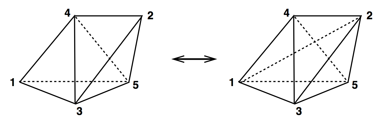
Here is what these ergodic moves look like in 3D. By choosing to make these moves according to the Metropolis-Hastings algorithm, we effectively sample all possible paths as the universe moves from one time step to the next.

Which is what the path integral is?

Exactly.

So, these are the moves which sample all possible (2+1) dimensional discretized universes.

So how do we use these moves?

First, let's start by generating a random, foliated triangulation with $n$ simplices and $t$ timeslices. Here is a program to do that.

A foliated triangulation is a Delaunay triangulation with two criteria:

1. Each vertex has a time value
2. Each simplex contains vertices that differ by at most one time value

In (2+1) dimensions, then, we are dealing with simplices that have 4 vertices (an n-dimensional simplex always has n+1 vertices).

We can thus classify the (2+1) dimensional simplex as a (3,1) simplex (3 vertices on the low timeslice and one vertex on the high timeslice), a (2,2) simplex, or a (1,3) simplex.

Likewise, we can name the moves similarly.

The top move takes a (3,1) simplex and a (2,2) simplex and converts it to a (3,1) simplex plus two (2,2) simplices. This is called a (2,3) move, and its reverse is naturally a (3,2) move.

The middle move takes a (1,3) simplex and a (3,1) simplex and converts it to three (1,3) simplices plus three (3,1) simplices. This is a (2,6) move along with the reverse (6,2) move.

The bottom move takes two (1,3) simplices and two (3,1) simplices and makes different (1,3) and (3,1) simplices. This is called a (4,4) move, and it is its own reverse.

The CDT action is then based on the Regge action:

$$ \begin{aligned} S^{(3)} &= 2\pi k\sqrt{\alpha}N_1^{TL} + N_3^{(3,1)}\left[ -3k\operatorname{arcsinh}\left(\frac{1}{\sqrt{3}\sqrt{4\alpha+1}}\right) -3k\sqrt{\alpha}\operatorname{arccos}\left(\frac{2\alpha+1}{4\alpha+1}\right) -\frac{\lambda}{12}\sqrt{3\alpha+1}\right] \ &\quad + N_3^{(2,2)}\left[ 2k\operatorname{arcsinh}\left(\frac{2\sqrt{4\alpha+2}}{4\alpha+1}\right) -4k\sqrt{\alpha}\operatorname{arccos}\left(-\frac{1}{4\alpha+1}\right) -\frac{\lambda}{12}\sqrt{4\alpha+2}\right] \end{aligned} $$

This formula is the Regge action with some trigonometric identities applied after taking the length of spacelike edges to be 1 and the length of timelike edges to be $\alpha$. There are a few more constants thrown in for good measure.⁴

However complex this looks, it generates a number.

Metropolis-Hastings then calculates the probability of making a move as:

$$ P=a_{1}a_{2}$$

Where:

$$ a_{1}=\frac{\text{move}[i]}{\sum_i\text{move}[i]} $$

And:

$$ a_{2}=e^{\Delta S} $$

$a_{1}$ is essentially the probability of making $\text{move}[i]$ versus making all other moves, and $a_{2}$ is the change in the action caused by making $\text{move}[i]$.

This comes from the fact that we are using Markov chains, which forget all history except the previous move,⁵ and the principle of detailed balance, which states that the probability of transitioning from $x\rightarrow x\prime$ equals the probability of $x\prime\rightarrow x$.

$a_{1}$ is easy to calculate: you just keep track of the total successful moves of each type.

$a_{2}$ is likewise simple:

• A (2,3) move will change $N_1^{TL}$ and $N_3^{(2,2)}$ by +1 each; a (3,2) by -1 each.

• A (2,6) move changes $N_3^{(3,1)}$ by +4 and $N_1^{TL}$ by +2; a (6,2) by -4 and -2 respectively.

• A (4,4) move doesn't change the action at all; $a_2 = 1$, and only $a_1$ is needed.

By attempting a large number of moves, some of which will be accepted⁶ and some of which will be rejected, we can approximate the distribution thus producing an ensemble.

Now what?

Now we can collect data on the various ensembles, and obtain things like spectral dimension, transition amplitudes, or in my case, the Newtonian Limit.

So that's the backstory (modulo some digressions).

To have results before, well, the end of the universe, we should use a fast language, e.g. C++ together with a battle-tested library capable of manipulating Delaunay triangulations in various dimensions, e.g. CGAL.⁷

Of course, that isn't enough, we have to write good code too. Thinking about the problem statement (that we've spent most of this post on) conjures up GoF patterns such as the Command Pattern, the Strategy Pattern, plus the Producer-consumer problem.

All which seem to have well tested, elegant solutions.

But isn't functional programming the old/new hotness?

We'll get into that next time!

You didn't actually address the title of this post.

I do need to sleep sometime.

Fair enough.